what assumptions had to be made for you to use student’s t-distribution

Statistical hypothesis test

The t-test is any statistical hypothesis exam in which the test statistic follows a Pupil's t-distribution under the cipher hypothesis.

A t-test is the near normally applied when the test statistic would follow a normal distribution if the value of a scaling term in the test statistic were known. When the scaling term is unknown and is replaced by an gauge based on the data, the exam statistics (under certain conditions) follow a Educatee'south t distribution. The t-test can be used, for example, to determine if the means of two sets of data are significantly different from each other.

History [edit]

The term "t-statistic" is abbreviated from "hypothesis test statistic".^[ane] In statistics, the t-distribution was outset derived as a posterior distribution in 1876 past Helmert^{[ii] [iii] [4]} and Lüroth.^{[five] [six] [7]} The t-distribution besides appeared in a more general form as Pearson Type IV distribution in Karl Pearson's 1895 paper.^[8] Even so, the T-Distribution, as well known equally Pupil's t-distribution, gets its name from William Sealy Gosset who get-go published information technology in English in 1908 in the scientific journal Biometrika using his pseudonym "Educatee"^{[9] [10]} because his employer preferred staff to use pen names when publishing scientific papers instead of their real proper noun, so he used the name "Educatee" to hide his identity.^[11] Gosset worked at the Guinness Brewery in Dublin, Ireland, and was interested in the problems of small samples – for instance, the chemic properties of barley with small sample sizes. Hence a second version of the etymology of the term Student is that Guinness did not want their competitors to know that they were using the t-examination to determine the quality of raw cloth (see Student's t-distribution for a detailed history of this pseudonym, which is non to exist confused with the literal term student). Although it was William Gosset after whom the term "Student" is penned, it was actually through the work of Ronald Fisher that the distribution became well known as "Student'due south distribution"^[12] and "Student's t-test".

Gosset had been hired owing to Claude Guinness'south policy of recruiting the best graduates from Oxford and Cambridge to apply biochemistry and statistics to Guinness's industrial processes.^[13] Gosset devised the t-test as an economical way to monitor the quality of stout. The t-test work was submitted to and accustomed in the periodical Biometrika and published in 1908.^[14]

Guinness had a policy of allowing technical staff leave for report (and then-chosen "study leave"), which Gosset used during the first two terms of the 1906–1907 academic year in Professor Karl Pearson's Biometric Laboratory at University College London.^[15] Gosset's identity was then known to fellow statisticians and to editor-in-chief Karl Pearson.^[16]

Uses [edit]

Among the most frequently used t-tests are:

• A one-sample location test of whether the mean of a population has a value specified in a nothing hypothesis.
• A 2-sample location test of the aught hypothesis such that the ways of 2 populations are equal. All such tests are unremarkably called Student's t-tests, though strictly speaking that name should only exist used if the variances of the two populations are likewise assumed to be equal; the grade of the test used when this assumption is dropped is sometimes called Welch'south t-test. These tests are oftentimes referred to equally unpaired or independent samples t-tests, equally they are typically applied when the statistical units underlying the two samples being compared are non-overlapping.^[17]

Assumptions [edit]

Nigh exam statistics take the form t = Z / s , where Z and s are functions of the data.

Z may exist sensitive to the alternative hypothesis (i.e., its magnitude tends to be larger when the alternative hypothesis is truthful), whereas s is a scaling parameter that allows the distribution of t to be determined.

Every bit an case, in the one-sample t-test

${\displaystyle t={\frac {Z}{due south}}={\frac {{\bar {X}}-\mu }{{\widehat {\sigma }}/{\sqrt {n}}}}}$

where X is the sample hateful from a sample X _i, X ₂, …, X _n , of size northward , s is the standard error of the hateful, ${\textstyle {\widehat {\sigma }}}$ is the estimate of the standard departure of the population, and μ is the population mean.

The assumptions underlying a t-test in the simplest class above are that:

• X follows a normal distribution with mean μ and variance σ ² / north
• s ²(n − ane)/σ ² follows a χ ² distribution with due north − 1 degrees of freedom. This assumption is met when the observations used for estimating due south ² come up from a normal distribution (and i.i.d for each group).
• Z and s are contained.

In the t-exam comparing the means of 2 independent samples, the following assumptions should be met:

• The means of the two populations being compared should follow normal distributions. Under weak assumptions, this follows in large samples from the primal limit theorem, even when the distribution of observations in each group is non-normal.^[18]
• If using Pupil'south original definition of the t-test, the two populations being compared should have the aforementioned variance (testable using F-test, Levene'due south exam, Bartlett's test, or the Chocolate-brown–Forsythe test; or assessable graphically using a Q–Q plot). If the sample sizes in the two groups being compared are equal, Student's original t-exam is highly robust to the presence of unequal variances.^[19] Welch's t-examination is insensitive to equality of the variances regardless of whether the sample sizes are similar.
• The data used to acquit out the exam should either be sampled independently from the two populations being compared or be fully paired. This is in general not testable from the information, but if the data are known to exist dependent (e.g. paired by examination design), a dependent test has to exist applied. For partially paired data, the classical independent t-tests may give invalid results every bit the test statistic might not follow a t distribution, while the dependent t-examination is sub-optimal as information technology discards the unpaired information.^[20]

About two-sample t-tests are robust to all but large deviations from the assumptions.^[21]

For exactness, the t-test and Z-examination require normality of the sample ways, and the t-test additionally requires that the sample variance follows a scaled χ ² distribution, and that the sample hateful and sample variance be statistically independent. Normality of the individual information values is not required if these conditions are met. By the primal limit theorem, sample ways of moderately large samples are often well-approximated past a normal distribution fifty-fifty if the data are non usually distributed. For non-normal information, the distribution of the sample variance may deviate substantially from a χ ² distribution.

However, if the sample size is big, Slutsky's theorem implies that the distribution of the sample variance has piffling effect on the distribution of the test statistic. That is every bit sample size ${\displaystyle n}$ increases:

Unpaired and paired 2-sample t-tests [edit]

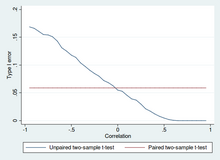
Blazon I error of unpaired and paired two-sample t-tests as a function of the correlation. The simulated random numbers originate from a bivariate normal distribution with a variance of 1. The significance level is 5% and the number of cases is threescore.

Power of unpaired and paired two-sample t-tests as a office of the correlation. The imitation random numbers originate from a bivariate normal distribution with a variance of 1 and a departure of the expected value of 0.4. The significance level is 5% and the number of cases is 60.

Ii-sample t-tests for a difference in hateful involve independent samples (unpaired samples) or paired samples. Paired t-tests are a form of blocking, and accept greater ability (probability of fugitive a type II error, also known equally a false negative) than unpaired tests when the paired units are like with respect to "racket factors" that are independent of membership in the two groups being compared.^[22] In a different context, paired t-tests tin can be used to reduce the effects of confounding factors in an observational study.

Contained (unpaired) samples [edit]

The independent samples t-test is used when two separate sets of independent and identically distributed samples are obtained, and one variable from each of the two populations is compared. For example, suppose nosotros are evaluating the upshot of a medical treatment, and we enroll 100 subjects into our report, then randomly assign 50 subjects to the handling grouping and 50 subjects to the control group. In this case, we accept 2 independent samples and would use the unpaired form of the t-test.

Paired samples [edit]

Paired samples t-tests typically consist of a sample of matched pairs of similar units, or ane group of units that has been tested twice (a "repeated measures" t-test).

A typical case of the repeated measures t-exam would be where subjects are tested prior to a handling, say for high claret pressure, and the same subjects are tested again after treatment with a blood-pressure-lowering medication. By comparing the aforementioned patient'south numbers earlier and after treatment, nosotros are finer using each patient as their own control. That way the correct rejection of the null hypothesis (hither: of no difference made by the treatment) can go much more likely, with statistical power increasing simply because the random interpatient variation has now been eliminated. Still, an increase of statistical power comes at a price: more tests are required, each subject having to be tested twice. Because half of the sample at present depends on the other one-half, the paired version of Pupil's t-exam has simply n / 2 − ane degrees of freedom (with n existence the total number of observations). Pairs become individual test units, and the sample has to be doubled to achieve the same number of degrees of liberty. Commonly, there are n − i degrees of freedom (with n being the total number of observations).^[23]

A paired samples t-test based on a "matched-pairs sample" results from an unpaired sample that is subsequently used to form a paired sample, by using additional variables that were measured along with the variable of involvement.^[24] The matching is carried out by identifying pairs of values consisting of one observation from each of the two samples, where the pair is similar in terms of other measured variables. This arroyo is sometimes used in observational studies to reduce or eliminate the furnishings of confounding factors.

Paired samples t-tests are often referred to as "dependent samples t-tests".

Calculations [edit]

Explicit expressions that tin be used to carry out various t-tests are given below. In each case, the formula for a test statistic that either exactly follows or closely approximates a t-distribution nether the null hypothesis is given. Also, the appropriate degrees of liberty are given in each case. Each of these statistics tin can be used to carry out either a one-tailed or 2-tailed test.

In one case the t value and degrees of freedom are determined, a p-value can be found using a tabular array of values from Student's t-distribution. If the calculated p-value is below the threshold chosen for statistical significance (normally the 0.10, the 0.05, or 0.01 level), then the null hypothesis is rejected in favor of the alternative hypothesis.

1-sample t-test [edit]

In testing the null hypothesis that the sample hateful is equal to a specified value μ ₀ , one uses the statistic

${\displaystyle t={\frac {{\bar {x}}-\mu _{0}}{s/{\sqrt {n}}}}}$

where ${\displaystyle {\bar {10}}}$ is the sample hateful, s is the sample standard divergence and n is the sample size. The degrees of liberty used in this test are due north − one. Although the parent population does not need to be normally distributed, the distribution of the population of sample means ${\displaystyle {\bar {ten}}}$ is assumed to be normal.

By the central limit theorem, if the observations are contained and the second moment exists, and so ${\displaystyle t}$ will be approximately normal Northward(0;1).

Slope of a regression line [edit]

Suppose ane is plumbing fixtures the model

${\displaystyle Y=\alpha +\beta ten+\varepsilon }$

where ten is known, α and β are unknown, ε is a normally distributed random variable with mean 0 and unknown variance σ ⁱⁱ , and Y is the outcome of interest. Nosotros want to examination the nada hypothesis that the gradient β is equal to some specified value β ₀ (oftentimes taken to exist 0, in which instance the nil hypothesis is that 10 and y are uncorrelated).

Let

${\displaystyle {\brainstorm{aligned}{\widehat {\alpha }},{\widehat {\beta }}&={\text{least-squares estimators}},\\SE_{\widehat {\blastoff }},SE_{\widehat {\beta }}&={\text{the standard errors of least-squares estimators}}.\end{aligned}}}$

And so

${\displaystyle t_{\text{score}}={\frac {{\widehat {\beta }}-\beta _{0}}{SE_{\widehat {\beta }}}}\sim {\mathcal {T}}_{due north-two}}$

has a t-distribution with n − 2 degrees of freedom if the null hypothesis is true. The standard error of the slope coefficient:

${\displaystyle SE_{\widehat {\beta }}={\frac {\sqrt {{\dfrac {1}{due north-2}}\displaystyle \sum _{i=i}^{n}\left(y_{i}-{\widehat {y}}_{i}\right)^{ii}}}{\sqrt {\displaystyle \sum _{i=1}^{n}\left(x_{i}-{\bar {10}}\correct)^{2}}}}}$

tin be written in terms of the residuals. Allow

${\displaystyle {\begin{aligned}{\widehat {\varepsilon }}_{i}&=y_{i}-{\widehat {y}}_{i}=y_{i}-\left({\widehat {\alpha }}+{\widehat {\beta }}x_{i}\correct)={\text{residuals}}={\text{estimated errors}},\\{\text{SSR}}&=\sum _{i=one}^{n}{{\widehat {\varepsilon }}_{i}}^{2}={\text{sum of squares of residuals}}.\end{aligned}}}$

So t _score is given by:

${\displaystyle t_{\text{score}}={\frac {\left({\widehat {\beta }}-\beta _{0}\right){\sqrt {north-two}}}{\sqrt {\frac {SSR}{\sum _{i=1}^{n}\left(x_{i}-{\bar {x}}\right)^{2}}}}}.}$

Another way to determine the t _score is:

${\displaystyle t_{\text{score}}={\frac {r{\sqrt {northward-2}}}{\sqrt {ane-r^{two}}}},}$

where r is the Pearson correlation coefficient.

The t _{score, intercept} can be determined from the t _{score, gradient}:

${\displaystyle t_{\text{score,intercept}}={\frac {\blastoff }{\beta }}{\frac {t_{\text{score,slope}}}{\sqrt {s_{\text{x}}^{2}+{\bar {x}}^{2}}}}}$

where s _x ² is the sample variance.

Independent two-sample t-test [edit]

Equal sample sizes and variance [edit]

Given two groups (1, two), this test is only applicative when:

• the two sample sizes (that is, the number n of participants of each group) are equal;
• it tin can be assumed that the two distributions have the same variance;

Violations of these assumptions are discussed below.

The t statistic to exam whether the means are different can be calculated as follows:

${\displaystyle t={\frac {{\bar {X}}_{1}-{\bar {X}}_{2}}{s_{p}{\sqrt {\frac {ii}{n}}}}}}$

where

${\displaystyle s_{p}={\sqrt {\frac {s_{X_{1}}^{two}+s_{X_{2}}^{2}}{2}}}.}$

Here south_p is the pooled standard departure for n = n _one = n _ii and southward  ^two
_{X ane} and s  ²
_{Ten 2} are the unbiased estimators of the variances of the two samples. The denominator of t is the standard error of the difference between two means.

For significance testing, the degrees of freedom for this test is 2due north − ii where n is the number of participants in each group.

Equal or unequal sample sizes, similar variances ( 1 / 2 < southward _{X ane} / s _{X ii} < 2) [edit]

This examination is used only when it tin can exist causeless that the two distributions accept the same variance. (When this assumption is violated, encounter beneath.) The previous formulae are a special case of the formulae below, ane recovers them when both samples are equal in size: n = northward _ane = due north ₂ .

The t statistic to examination whether the means are different can exist calculated as follows:

${\displaystyle t={\frac {{\bar {X}}_{one}-{\bar {X}}_{2}}{s_{p}\cdot {\sqrt {{\frac {1}{n_{1}}}+{\frac {1}{n_{2}}}}}}}}$

where

${\displaystyle s_{p}={\sqrt {\frac {\left(n_{one}-1\right)s_{X_{1}}^{2}+\left(n_{2}-1\right)s_{X_{2}}^{2}}{n_{1}+n_{2}-2}}}}$

is an computer of the pooled standard deviation of the two samples: information technology is defined in this way so that its foursquare is an unbiased computer of the common variance whether or not the population means are the same. In these formulae, n_i − 1 is the number of degrees of liberty for each group, and the total sample size minus two (that is, north ₁ + due north ₂ − 2) is the full number of degrees of freedom, which is used in significance testing.

Equal or diff sample sizes, unequal variances (s _{X ane} > iis _{X ii} or due south _{Ten 2} > 2s _{X one} ) [edit]

This exam, as well known as Welch's t-examination, is used only when the two population variances are not assumed to be equal (the two sample sizes may or may not be equal) and hence must exist estimated separately. The t statistic to test whether the population means are different is calculated equally:

${\displaystyle t={\frac {{\bar {X}}_{1}-{\bar {X}}_{2}}{s_{\bar {\Delta }}}}}$

where

${\displaystyle s_{\bar {\Delta }}={\sqrt {{\frac {s_{1}^{two}}{n_{1}}}+{\frac {s_{two}^{2}}{n_{2}}}}}.}$

Here south_i ⁱⁱ is the unbiased calculator of the variance of each of the two samples with n_i = number of participants in group i ( i = 1 or 2). In this case ${\textstyle (s_{\bar {\Delta }})^{2}}$ is non a pooled variance. For use in significance testing, the distribution of the test statistic is approximated every bit an ordinary Pupil's t-distribution with the degrees of freedom calculated using

${\displaystyle \mathrm {d.f.} ={\frac {\left({\frac {s_{1}^{ii}}{n_{ane}}}+{\frac {s_{2}^{2}}{n_{two}}}\correct)^{two}}{{\frac {\left(s_{1}^{2}/n_{i}\right)^{2}}{n_{1}-ane}}+{\frac {\left(s_{two}^{ii}/n_{2}\right)^{2}}{n_{2}-1}}}}.}$

This is known as the Welch–Satterthwaite equation. The true distribution of the test statistic actually depends (slightly) on the two unknown population variances (meet Behrens–Fisher problem).

Dependent t-test for paired samples [edit]

This test is used when the samples are dependent; that is, when there is only one sample that has been tested twice (repeated measures) or when at that place are two samples that have been matched or "paired". This is an example of a paired divergence test. The t statistic is calculated as

${\displaystyle t={\frac {{\bar {X}}_{D}-\mu _{0}}{s_{D}/{\sqrt {n}}}}}$

where ${\displaystyle {\bar {10}}_{D}}$ and ${\displaystyle s_{D}}$ are the average and standard deviation of the differences between all pairs. The pairs are due east.m. either one person'south pre-test and post-examination scores or between-pairs of persons matched into meaningful groups (for instance drawn from the same family unit or age group: see table). The abiding μ ₀ is zippo if we want to examination whether the average of the divergence is significantly different. The caste of liberty used is n − one, where due north represents the number of pairs.

Example of repeated measures

Number	Name	Test one	Test two
1	Mike	35%	67%
two	Melanie	fifty%	46%
3	Melissa	90%	86%
four	Mitchell	78%	91%

Instance of matched pairs

Pair	Name	Historic period	Test
i	John	35	250
1	Jane	36	340
2	Jimmy	22	460
2	Jessy	21	200

Worked examples [edit]

Let A _ane denote a set obtained by drawing a random sample of six measurements:

${\displaystyle A_{1}=\{30.02,\ 29.99,\ 30.xi,\ 29.97,\ 30.01,\ 29.99\}}$

and permit A ₂ denote a second set obtained similarly:

${\displaystyle A_{2}=\{29.89,\ 29.93,\ 29.72,\ 29.98,\ 30.02,\ 29.98\}}$

These could be, for example, the weights of screws that were chosen out of a bucket.

Nosotros will acquit out tests of the null hypothesis that the means of the populations from which the two samples were taken are equal.

The difference betwixt the two sample means, each denoted by 10 _i , which appears in the numerator for all the two-sample testing approaches discussed above, is

${\displaystyle {\bar {X}}_{one}-{\bar {X}}_{two}=0.095.}$

The sample standard deviations for the two samples are approximately 0.05 and 0.11, respectively. For such pocket-sized samples, a test of equality between the two population variances would not exist very powerful. Since the sample sizes are equal, the two forms of the 2-sample t-test volition perform similarly in this example.

Unequal variances [edit]

If the approach for diff variances (discussed higher up) is followed, the results are

${\displaystyle {\sqrt {{\frac {s_{one}^{2}}{n_{1}}}+{\frac {s_{two}^{2}}{n_{2}}}}}\approx 0.04849}$

and the degrees of liberty

${\displaystyle {\text{d.f.}}\approx 7.031.}$

The test statistic is approximately ane.959, which gives a two-tailed test p-value of 0.09077.

Equal variances [edit]

If the approach for equal variances (discussed in a higher place) is followed, the results are

${\displaystyle s_{p}\approx 0.08396}$

and the degrees of liberty

${\displaystyle {\text{d.f.}}=10.}$

The examination statistic is approximately equal to ane.959, which gives a 2-tailed p-value of 0.07857.

[edit]

Alternatives to the t-test for location problems [edit]

The t-test provides an verbal examination for the equality of the means of 2 i.i.d. normal populations with unknown, merely equal, variances. (Welch's t-test is a about exact exam for the case where the data are normal simply the variances may differ.) For moderately big samples and a one tailed test, the t-test is relatively robust to moderate violations of the normality supposition.^[25] In large enough samples, the t-examination asymptotically approaches the z-test, and becomes robust even to large deviations from normality.^[xviii]

If the information are substantially non-normal and the sample size is small, the t-test tin give misleading results. See Location test for Gaussian calibration mixture distributions for some theory related to i item family of not-normal distributions.

When the normality assumption does not concur, a non-parametric alternative to the t-test may take better statistical ability. All the same, when data are non-normal with differing variances between groups, a t-test may have better type-ane error command than some non-parametric alternatives.^[26] Furthermore, not-parametric methods, such as the Mann-Whitney U examination discussed below, typically do non test for a difference of means, and so should exist used carefully if a difference of means is of primary scientific interest.^[18] For instance, Isle of man-Whitney U test will go along the type one fault at the desired level blastoff if both groups have the same distribution. It will also take power in detecting an alternative past which group B has the same distribution as A but afterward some shift by a constant (in which case there would indeed exist a departure in the ways of the two groups). Nevertheless, there could be cases where grouping A and B will have unlike distributions but with the same means (such as two distributions, ane with positive skewness and the other with a negative one, simply shifted so to have the aforementioned means). In such cases, MW could take more than alpha level ability in rejecting the Null hypothesis merely attributing the interpretation of difference in means to such a result would be incorrect.

In the presence of an outlier, the t-test is not robust. For example, for ii contained samples when the information distributions are disproportionate (that is, the distributions are skewed) or the distributions have big tails, then the Wilcoxon rank-sum test (besides known as the Isle of mann–Whitney U test) can accept three to four times higher power than the t-test.^{[25] [27] [28]} The nonparametric counterpart to the paired samples t-exam is the Wilcoxon signed-rank exam for paired samples. For a discussion on choosing betwixt the t-exam and nonparametric alternatives, encounter Lumley, et al. (2002).^[18]

One-way assay of variance (ANOVA) generalizes the two-sample t-exam when the data vest to more than two groups.

A design which includes both paired observations and independent observations [edit]

When both paired observations and independent observations are nowadays in the two sample design, bold data are missing completely at random (MCAR), the paired observations or independent observations may be discarded in guild to go on with the standard tests higher up. Alternatively making use of all of the available data, assuming normality and MCAR, the generalized partially overlapping samples t-test could be used.^[29]

Multivariate testing [edit]

A generalization of Student's t statistic, called Hotelling's t-squared statistic, allows for the testing of hypotheses on multiple (often correlated) measures inside the aforementioned sample. For instance, a researcher might submit a number of subjects to a personality test consisting of multiple personality scales (e.g. the Minnesota Multiphasic Personality Inventory). Because measures of this type are usually positively correlated, it is not advisable to conduct separate univariate t-tests to test hypotheses, as these would neglect the covariance among measures and inflate the take chances of falsely rejecting at least one hypothesis (Type I fault). In this example a single multivariate examination is preferable for hypothesis testing. Fisher'southward Method for combining multiple tests with alpha reduced for positive correlation amongst tests is one. Another is Hotelling's T ² statistic follows a T ² distribution. Still, in practice the distribution is rarely used, since tabulated values for T ^two are hard to observe. Commonly, T ² is converted instead to an F statistic.

For a one-sample multivariate test, the hypothesis is that the mean vector ( μ ) is equal to a given vector ( μ ₀ ). The test statistic is Hotelling's t ² :

${\displaystyle t^{2}=n({\bar {\mathbf {x} }}-{{\boldsymbol {\mu }}_{0}})'{\mathbf {S} }^{-i}({\bar {\mathbf {x} }}-{{\boldsymbol {\mu }}_{0}})}$

where north is the sample size, ten is the vector of column means and S is an yard × m sample covariance matrix.

For a two-sample multivariate exam, the hypothesis is that the mean vectors ( μ ₁, μ _ii ) of two samples are equal. The test statistic is Hotelling'southward ii-sample t ^two :

${\displaystyle t^{2}={\frac {n_{1}n_{2}}{n_{1}+n_{ii}}}\left({\bar {\mathbf {x} }}_{one}-{\bar {\mathbf {x} }}_{2}\right)'{\mathbf {S} _{\text{pooled}}}^{-one}\left({\bar {\mathbf {x} }}_{1}-{\bar {\mathbf {x} }}_{2}\correct).}$

Software implementations [edit]

Many spreadsheet programs and statistics packages, such as QtiPlot, LibreOffice Calc, Microsoft Excel, SAS, SPSS, Stata, DAP, gretl, R, Python, PSPP, MATLAB and Minitab, include implementations of Student's t-test.

Language/Programme	Function	Notes
Microsoft Excel pre 2010	TTEST(array1, array2, tails, type)	Run into [1]
Microsoft Excel 2010 and later	T.TEST(array1, array2, tails, blazon)	See [2]
LibreOffice Calc	TTEST(Data1; Data2; Style; Type)	Run into [3]
Google Sheets	TTEST(range1, range2, tails, type)	Come across [4]
Python	scipy.stats.ttest_ind(a, b, equal_var=True)	Encounter [v]
MATLAB	ttest(data1, data2)	Run across [6]
Mathematica	TTest[{data1,data2}]	Encounter [vii]
R	t.test(data1, data2, var.equal=TRUE)	See [8]
SAS	PROC TTEST	Meet [ix]
Java	tTest(sample1, sample2)	See [10]
Julia	EqualVarianceTTest(sample1, sample2)	Meet [xi]
Stata	ttest data1 == data2	Run into [12]

See also [edit]

• Conditional modify model
• F-test
• Noncentral t-distribution in power analysis
• Educatee'southward t-statistic
• Z-examination
• Isle of man–Whitney U test
• Šidák correction for t-test
• Welch's t-test
• Analysis of variance (ANOVA)

References [edit]

Citations [edit]

1. ^ The Microbiome in Health and Disease. Academic Press. 2020-05-29. p. 397. ISBN978-0-12-820001-viii.
2. ^ Szabó, István (2003), "Systeme aus einer endlichen Anzahl starrer Körper", Einführung in die Technische Mechanik, Springer Berlin Heidelberg, pp. 196–199, doi:10.1007/978-iii-642-61925-0_16, ISBN978-3-540-13293-vi
3. ^ Schlyvitch, B. (October 1937). "Untersuchungen über den anastomotischen Kanal zwischen der Arteria coeliaca und mesenterica superior und damit in Zusammenhang stehende Fragen". Zeitschrift für Anatomie und Entwicklungsgeschichte. 107 (6): 709–737. doi:10.1007/bf02118337. ISSN 0340-2061. S2CID 27311567.
4. ^ Helmert (1876). "Die Genauigkeit der Formel von Peters zur Berechnung des wahrscheinlichen Beobachtungsfehlers directer Beobachtungen gleicher Genauigkeit". Astronomische Nachrichten (in German). 88 (8–9): 113–131. Bibcode:1876AN.....88..113H. doi:10.1002/asna.18760880802.
5. ^ Lüroth, J. (1876). "Vergleichung von zwei Werthen des wahrscheinlichen Fehlers". Astronomische Nachrichten (in German). 87 (14): 209–220. Bibcode:1876AN.....87..209L. doi:x.1002/asna.18760871402.
6. ^ Pfanzagl J, Sheynin O (1996). "Studies in the history of probability and statistics. XLIV. A forerunner of the t-distribution". Biometrika. 83 (4): 891–898. doi:10.1093/biomet/83.4.891. MR 1766040.
7. ^ Sheynin, Oscar (1995). "Helmert'due south work in the theory of errors". Archive for History of Verbal Sciences. 49 (ane): 73–104. doi:ten.1007/BF00374700. ISSN 0003-9519. S2CID 121241599.
8. ^ Pearson, Grand. (1895-01-01). "Contributions to the Mathematical Theory of Evolution. 2. Skew Variation in Homogeneous Fabric". Philosophical Transactions of the Royal Society A: Mathematical, Physical and Engineering Sciences. 186: 343–414 (374). doi:10.1098/rsta.1895.0010. ISSN 1364-503X
9. ^ "Student" William Sealy Gosset (1908). "The probable fault of a mean" (PDF). Biometrika. 6 (1): ane–25. doi:10.1093/biomet/6.i.1. hdl:10338.dmlcz/143545. JSTOR 2331554
10. ^ "T Table".
11. ^ Wendl MC (2016). "Pseudonymous fame". Science. 351 (6280): 1406. doi:10.1126/science.351.6280.1406. PMID 27013722
12. ^ Walpole, Ronald E. (2006). Probability & statistics for engineers & scientists. Myers, H. Raymond. (seventh ed.). New Delhi: Pearson. ISBN81-7758-404-nine. OCLC 818811849.
13. ^ O'Connor, John J.; Robertson, Edmund F., "William Sealy Gosset", MacTutor History of Mathematics archive, University of St Andrews
14. ^ "The Probable Mistake of a Mean" (PDF). Biometrika. vi (1): 1–25. 1908. doi:ten.1093/biomet/6.ane.1. hdl:10338.dmlcz/143545. Retrieved 24 July 2016.
15. ^ Raju, T. N. (2005). "William Sealy Gosset and William A. Silverman: Two 'Students' of Science". Pediatrics. 116 (3): 732–5. doi:ten.1542/peds.2005-1134. PMID 16140715. S2CID 32745754.
16. ^ Dodge, Yadolah (2008). The Curtailed Encyclopedia of Statistics. Springer Science & Business Media. pp. 234–235. ISBN978-0-387-31742-7.
17. ^ Fadem, Barbara (2008). High-Yield Behavioral Scientific discipline. High-Yield Series. Hagerstown, Doctor: Lippincott Williams & Wilkins. ISBN9781451130300.
18. ^ ^{a b c d} Lumley, Thomas; Diehr, Paula; Emerson, Scott; Chen, Lu (May 2002). "The Importance of the Normality Assumption in Large Public Health Data Sets". Almanac Review of Public Wellness. 23 (1): 151–169. doi:10.1146/annurev.publhealth.23.100901.140546. ISSN 0163-7525. PMID 11910059.
19. ^ Markowski, Carol A.; Markowski, Edward P. (1990). "Conditions for the Effectiveness of a Preliminary Test of Variance". The American Statistician. 44 (four): 322–326. doi:ten.2307/2684360. JSTOR 2684360.
20. ^ Guo, Beibei; Yuan, Ying (2017). "A comparative review of methods for comparing means using partially paired data". Statistical Methods in Medical Research. 26 (3): 1323–1340. doi:10.1177/0962280215577111. PMID 25834090. S2CID 46598415.
21. ^ Bland, Martin (1995). An Introduction to Medical Statistics. Oxford University Press. p. 168. ISBN978-0-19-262428-4.
22. ^ Rice, John A. (2006). Mathematical Statistics and Data Analysis (3rd ed.). Duxbury Advanced. ^{[ ISBN missing ]}
23. ^ Weisstein, Eric. "Student's t-Distribution". mathworld.wolfram.com.
24. ^ David, H. A.; Gunnink, Jason 50. (1997). "The Paired t Test Under Artificial Pairing". The American Statistician. 51 (1): 9–12. doi:10.2307/2684684. JSTOR 2684684.
25. ^ ^{a b} Sawilowsky, Shlomo S.; Blair, R. Clifford (1992). "A More Realistic Look at the Robustness and Type Ii Error Properties of the t Test to Departures From Population Normality". Psychological Message. 111 (2): 352–360. doi:x.1037/0033-2909.111.2.352.
26. ^ Zimmerman, Donald Westward. (January 1998). "Invalidation of Parametric and Nonparametric Statistical Tests by Concurrent Violation of Two Assumptions". The Journal of Experimental Educational activity. 67 (1): 55–68. doi:ten.1080/00220979809598344. ISSN 0022-0973.
27. ^ Blair, R. Clifford; Higgins, James J. (1980). "A Comparing of the Power of Wilcoxon'due south Rank-Sum Statistic to That of Student'due south t Statistic Nether Various Nonnormal Distributions". Journal of Educational Statistics. 5 (4): 309–335. doi:ten.2307/1164905. JSTOR 1164905.
28. ^ Fay, Michael P.; Proschan, Michael A. (2010). "Wilcoxon–Mann–Whitney or t-exam? On assumptions for hypothesis tests and multiple interpretations of decision rules". Statistics Surveys. 4: one–39. doi:x.1214/09-SS051. PMC2857732. PMID 20414472.
29. ^ Derrick, B; Toher, D; White, P (2017). "How to compare the means of two samples that include paired observations and independent observations: A companion to Derrick, Russ, Toher and White (2017)" (PDF). The Quantitative Methods for Psychology. 13 (2): 120–126. doi:10.20982/tqmp.thirteen.2.p120.

Sources [edit]

• O'Mahony, Michael (1986). Sensory Evaluation of Food: Statistical Methods and Procedures. CRC Press. p. 487. ISBN0-82477337-iii.
• Printing, William H.; Teukolsky, Saul A.; Vetterling, William T.; Flannery, Brian P. (1992). Numerical Recipes in C: The Art of Scientific Computing. Cambridge University Press. p. 616. ISBN0-521-43108-5.

Further reading [edit]

• Boneau, C. Alan (1960). "The effects of violations of assumptions underlying the t test". Psychological Bulletin. 57 (1): 49–64. doi:10.1037/h0041412. PMID 13802482.
• Edgell, Stephen E.; Noon, Sheila M. (1984). "Outcome of violation of normality on the t examination of the correlation coefficient". Psychological Bulletin. 95 (iii): 576–583. doi:10.1037/0033-2909.95.3.576.

External links [edit]

Wikiversity has learning resources about t-test

• "Student test", Encyclopedia of Mathematics, EMS Press, 2001 [1994]
• Trochim, William M.One thousand. "The T-Examination", Research Methods Knowledge Base, conjoint.ly
• Econometrics lecture (topic: hypothesis testing) on YouTube by Mark Thoma

wilsonhisee1967.blogspot.com

Source: https://en.wikipedia.org/wiki/Student%27s_t-test

Share this post